핸즈온 머신러닝
코딩관련깃허브
안녕하세요. 팀 언플(Team Unsolved Problem)의 Polar B 입니다!
오늘은 지난 시간 ‘결정 트리’에 이어서 ‘앙상블 학습과 랜덤 포레스트’를 공부해 보도록 하겠습니다.
[Hands-On ML] Chapter 6. Decision Tree
그럼, 시작하겠습니다!
기본설정
# 공통
import numpy as np
import os

# 일관된 출력을 위해 유사난수 초기화
np.random.seed(42)

# 맷플롯립 설정
%matplotlib inline
import matplotlib
import matplotlib.pyplot as plt
plt.rcParams['axes.labelsize'] = 14
plt.rcParams['xtick.labelsize'] = 12
plt.rcParams['ytick.labelsize'] = 12

# 한글출력
matplotlib.rc('font', family='NanumBarunGothic')
matplotlib.rcParams['axes.unicode_minus'] = False

# 작업할 디렉토리
PROJECT_ROOT_DIR = "C:\\Python\\MLPATH" ##파이썬 디렉토리 저장
CHAPTER_ID = "decision_trees"
IMAGE_PATH = os.path.join(PROJECT_ROOT_DIR, "images", CHAPTER_ID)

def image_path(fig_id, image_path_k2h=IMAGE_PATH):
    return os.path.join(image_path_k2h, fig_id) ##사진을 저장할 위치
복잡한 질문에 대해 대부분의 경우 전문가의 답보다 무작위로 선택된 수천명의 사람의 답을 모은 것이 일반적으로 더 낫습니다. 이 아이디어를 기반으로 나온 것이 앙상블 학습입니다.
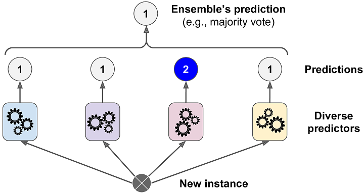 다수결 투표로 정해지는 분류기를 직접 투표 분류기(hard voting classifier) 라고 합니다.
각 분류기의 클래스 별 예측값의 확률을 가지고 평균을 내고, 평균이 가장 높은 클래스로 최종 앙상블 예측을 하는 분류기를 간접투표(soft voting classifier) (개별 모형의 조건부 확률의 합 기준) 라고 합니다.
예를들어 이 경우에는
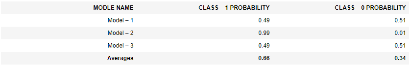
hard voting으로 한다면 0이라고 분류할 것이고, soft voting으로 한다면 1이라고 분류할 것입니다.
각 분류기가 약한 학습기(weak learner) (랜덤 추측보다 조금 더 높은 성은을 내는 분류기) 일지라도 충분하게 많고 다양하다면 강한 학습기(string learner) 가 될 수 있습니다.
다음 예제가 이같이 되는 이유를 설명해 줍니다.
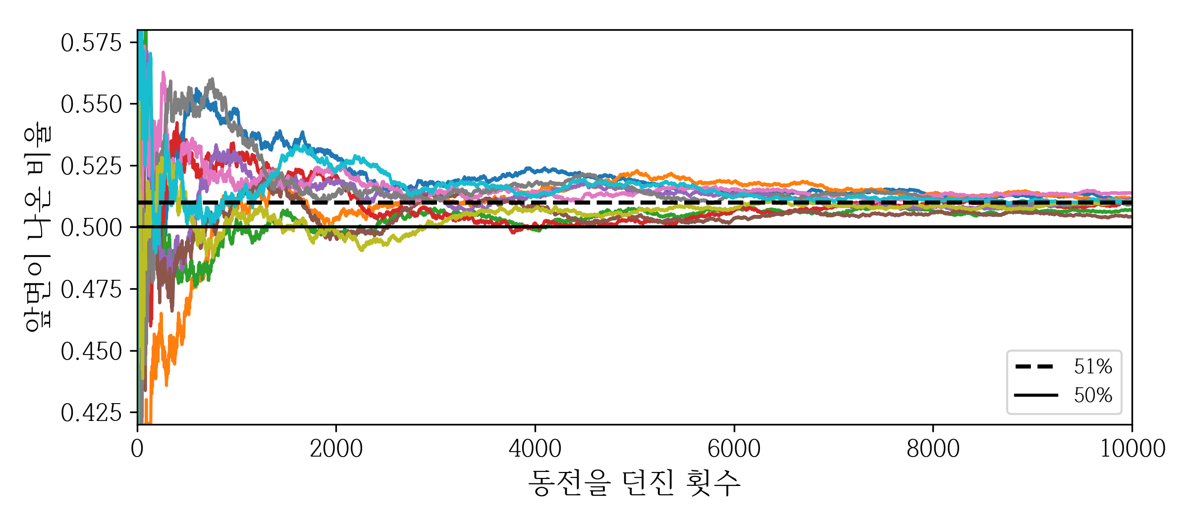
어떤 동전을 던졌을 때 앞면이 51%, 뒷면이 49% 나온다고 가정하겠습니다. 이 동전을 1000번 던지면 앞면은 대략 510번, 뒷면은 대략 490번이 나올 것이므로 다수는 앞면이 됩니다. 수학적으로 계산해보면 1000번을 던진 후 앞면이 다수가 될 확률은 75%에 가까워집니다.
(이항 분포의 확률 질량 함수로 계산한 값입니다. 확률이 p인 이항분포에서 n번의 시도 중 k번 성공할 확률은
\(Pr(K = k) = f(k;n,p) =
\begin{pmatrix}
n \\
k \\
\end{pmatrix}
p^k(1-p)^{n-k}\)
입니다. 동전을 던져 앞면이 1번만 나올 확률, 앞면이 2번만 나올 확률, . . ., 앞면이 499번만 나올 확률을 더해 1에서 빼면 1000번 던져 앞면이 절반 이상 나올 확률이 됩니다.)
책에서 이를 사이파이 모듈을 사용해 그래프로 보여주고있습니다.
import scipy.stats
1-scipy.stats.binom.cdf(499,1000,0.51)
0.7467502275561786 #결과
heads_proba = 0.51
coin_tosses = (np.random.rand(10000, 10) < heads_proba).astype(np.int32)
cumulative_heads_ratio = np.cumsum(coin_tosses, axis=0) / np.arange(1, 10001).reshape(-1, 1)

plt.figure(figsize=(8,3.5))
plt.plot(cumulative_heads_ratio)
plt.plot([0, 10000], [0.51, 0.51], "k--", linewidth=2, label="51%")
plt.plot([0, 10000], [0.5, 0.5], "k-", label="50%")
plt.xlabel("동전을 던진 횟수")
plt.ylabel("앞면이 나온 비율")
plt.legend(loc="lower right")
plt.axis([0, 10000, 0.42, 0.58])
save_fig("law_of_large_numbers_plot")
plt.show()
앙상블 방법은 예측기가 가능한 한 서로 독립적일 때 최고의 성능을 발휘합니다.
다음은 사이킷런의 투표 기반 분류기를 만들고 훈련시키는 코드입니다. (훈련 세트는 5장의 moons 데이터 셋입니다.)
from sklearn.model_selection import train_test_split
from sklearn.datasets import make_moons

X, y = make_moons(n_samples=500, noise=0.30, random_state=42)
X_train, X_test, y_train, y_test = train_test_split(X, y, random_state=42)
from sklearn.ensemble import RandomForestClassifier
from sklearn.ensemble import VotingClassifier
from sklearn.linear_model import LogisticRegression
from sklearn.svm import SVC

log_clf = LogisticRegression(solver='liblinear', random_state=42) ##로지스틱 회기
rnd_clf = RandomForestClassifier(n_estimators=10, random_state=42) ##랜덤 포레스트 분류기
svm_clf = SVC(gamma='auto', random_state=42) ## 서포트 벡터 분류기

## 분류기 앙상블을 만듦
voting_clf = VotingClassifier(
    estimators=[('lr', log_clf), ('rf', rnd_clf), ('svc', svm_clf)],
    voting='hard') # voting = 'hard' : 직접 투표

## 학습
voting_clf.fit(X_train, y_train)

## 정확성
from sklearn.metrics import accuracy_score

for clf in (log_clf, rnd_clf, svm_clf, voting_clf):  ## 각 분류기의 테스트셋 정확도 확인
    clf.fit(X_train, y_train)
    y_pred = clf.predict(X_test)
    print(clf.__class__.__name__, accuracy_score(y_test, y_pred))
LogisticRegression 0.864
RandomForestClassifier 0.872
SVC 0.888
VotingClassifier 0.896
log_clf = LogisticRegression(solver='liblinear', random_state=42)
rnd_clf = RandomForestClassifier(n_estimators=10, random_state=42)
svm_clf = SVC(gamma='auto', probability=True, random_state=42)

voting_clf = VotingClassifier(
    estimators=[('lr', log_clf), ('rf', rnd_clf), ('svc', svm_clf)],
    voting='soft')
voting_clf.fit(X_train, y_train)

from sklearn.metrics import accuracy_score

for clf in (log_clf, rnd_clf, svm_clf, voting_clf):
    clf.fit(X_train, y_train)
    y_pred = clf.predict(X_test)
    print(clf.__class__.__name__, accuracy_score(y_test, y_pred))
LogisticRegression 0.864
RandomForestClassifier 0.872
SVC 0.888
VotingClassifier 0.912
위 결과로 ‘어떤 모델이 무조건 더 좋다’라고 말할 수 없습니다. 데이터마다 다르며 적합한 모델을 찾기 위해선 전부 적용시켜보는 수밖에 없습니다.
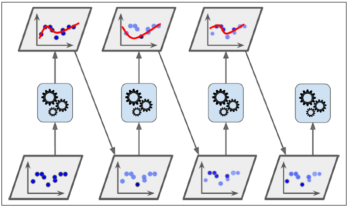
훈련 세트의 서브셋을 무작위로 구성하여 분류기를 각기 다르게 학습시키는 것입니다. 중복을 허용하여 샘플링을 하면 배깅(bootstrap aggregating의 줄임말), 중복을 허용하지 않고 샘플링을 하면 페이스팅(pasting) 이라고 합니다.
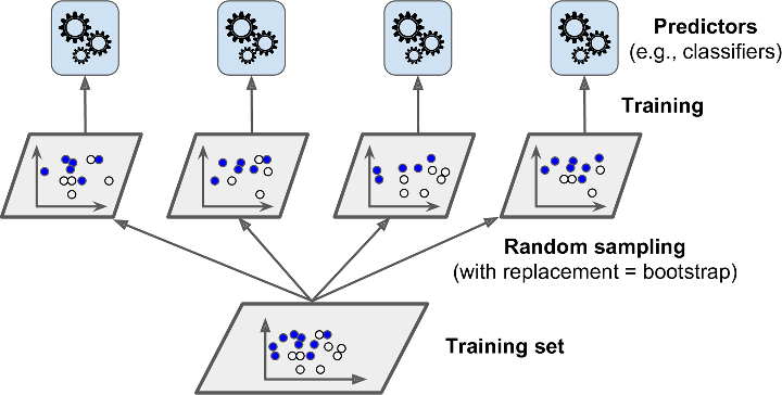
전형적으로 분류일 때는 통계적 최빈값(statistical mode) (가장 많은 예측 결과)을, 회귀에 대해서는 평균을 계산합니다
각 모델은 전체 학습 데이터 셋으로 학습시킨 것 보다 편향되어 있지만, 앙상블을 통해 편형과 분산이 감소합니다. 일반적으로 앙상블 학습은 전체 학습데이터 셋을 이용해 하나의 모델을 학습시킬 때와 비교해 편향은 비슷하지만 분산은 줄어듭니다.
(그림에서 볼 수 있듯이 예측기는 동시에 다른 CPU 코어나 서버에 병렬로 학습시킬 수 있습니다.)
moons 데이터를 그대로 사용해서 배깅과 페이스팅 모델을 구현합니다.
from sklearn.ensemble import BaggingClassifier
from sklearn.tree import DecisionTreeClassifier

## 결정트리 분류기 500개의 앙상블 훈련 코드
## 중복을 허용해서 (bootstrap = True), 무작위로 선택된(random_state=42) 100개의 샘플로 훈련(max_sample=100). 사용할 코어수(n_jobs = -1)
bag_clf = BaggingClassifier(
    DecisionTreeClassifier(random_state=42), n_estimators=500,
    max_samples=100, bootstrap=True, n_jobs=-1, random_state=42)
## 훈련
bag_clf.fit(X_train, y_train)
y_pred = bag_clf.predict(X_test)
## 정확도
from sklearn.metrics import accuracy_score
print(accuracy_score(y_test, y_pred))
0.904
BaggingClassifier는 base_estimator가 클래스 확률을 추정할 수 있으면(즉, predict_proba() 함수가 있으면) 직접투표대신 자동으로 간접투표방식을 사용합니다.
from sklearn.ensemble import BaggingClassifier
from sklearn.tree import DecisionTreeClassifier

## 결정트리 분류기 500개의 앙상블 훈련 코드
## 중복을 허용 안하고 (bootstrap = False), 무작위로 선택된(random_state=42) 100개의 샘플로 훈련(max_sample=100). 사용할 코어수(n_jobs = -1)
pas_clf = BaggingClassifier(
    DecisionTreeClassifier(random_state=42), n_estimators=500,
    max_samples=100, bootstrap=False, n_jobs=-1, random_state=42)
pas_clf.fit(X_train, y_train)
y_pred = bag_clf.predict(X_test)

from sklearn.metrics import accuracy_score
print(accuracy_score(y_test, y_pred))
0.912
배깅에서 중복을 허용(bootstrap=True)하여 훈련세트의 크기만큼 m개의 샘플을 선택합니다. 이는 평균적으로 데이터 셋의 63%정도만 샘플링 된다는 것을 의미합니다. 이때 나머지 선택되지 않은 나머지 37%를 oob(out-of-bag) 샘플이라고 부릅니다. 그리고 이 oob샘플을 사용해 모델을 평가하는 것을 oob평가라고 합니다.
선택되지 않을 확률이 왜 37%가 나오는가 궁금하신 분은 아래의 포스트를 참고하시기 바랍니다.
랜덤 포레스트에서 어떤 데이터 포인트가 부트스트랩 샘플에 포함되지 않을 확률
코드로는 아래와 같이 확인할 수 있습니다.
bag_clf = BaggingClassifier(
    DecisionTreeClassifier(random_state=42), n_estimators=500,
    max_samples=100, bootstrap=True, n_jobs=-1, random_state=42, oob_score=True)
bag_clf.fit(X_train, y_train)
y_pred = bag_clf.predict(X_test)

bag_clf.oob_score_
0.9253333333333333
BaggingClassifier는 특성(feature) 샘플링 또한 max_features와 bootstrap_features 두 개의 인자를 통해 제공합니다. 위의 두 인자를 이용해 각 모델은 랜덤하게 선택한 특성(feature)으로 학습하게 됩니다.
이러한 방법은 데이터의 특성이 많은 고차원의 데이터셋을 다룰 때 적절합니다. 학습 데이터 셋의 특성 및 샘플링(bootstraping) 사용 유무에 따라 두 종류로 나눌 수 있습니다.
이러한 특성 샘플링은 더 다양한 모델을 만들며 편향은 늘어나지만 분산을 낮출 수 있습니다.
bag_clf = BaggingClassifier(
    DecisionTreeClassifier(random_state=42), n_estimators=500,
    max_samples=100, bootstrap=True, n_jobs=-1, random_state=42,    # bootstrap을 False로 하면
    max_features = 0.5, bootstrap_features=True)                    # 랜덤 서브스페이스
bag_clf.fit(X_train, y_train)
y_pred = bag_clf.predict(X_test)

from sklearn.metrics import accuracy_score
print(accuracy_score(y_test, y_pred))
0.864
배깅 분류기와 랜덤 포레스트 분류기를 비교해 보겠습니다.
##배깅 분류기
bag_clf = BaggingClassifier(
    DecisionTreeClassifier(splitter="random", max_leaf_nodes=16, random_state=42),
    n_estimators=500, max_samples=1.0, bootstrap=True, n_jobs=-1, random_state=42)

bag_clf.fit(X_train, y_train)
y_pred = bag_clf.predict(X_test)
##랜덤 포레스트 분류기
from sklearn.ensemble import RandomForestClassifier

rnd_clf = RandomForestClassifier(n_estimators=500, max_leaf_nodes=16, n_jobs=-1, random_state=42)
rnd_clf.fit(X_train, y_train)

y_pred_rf = rnd_clf.predict(X_test)
##두 모델의 예측 비교
np.sum(y_pred == y_pred_rf) / len(y_pred)  # 거의 동일한 예측
0.976
랜덤 포레스트는 트리를 생성할 때, 각 노드는 랜덤하게 특성(feature)의 서브셋을 만들어 분할합니다.
익스트림 랜덤 트리(Extremely Randomized Trees) 혹은 엑스트라 트리(Extra-Trees)는 트리를 더욱 무작위하게 만들기 위해 (보통의 결정 트리처럼 엔트로피나 불순도를 이용해) 최적의 임곗값을 찾는 대신 후보 특성을 사용해 무작위로 분할한 다음 그 중에서 최상의 분할을 선택합니다.
from sklearn.ensemble import ExtraTreesClassifier

extra_clf = ExtraTreesClassifier(n_estimators=500, max_leaf_nodes=16, n_jobs=-1, random_state=42)
extra_clf.fit(X_train, y_train)
y_pred_ext = extra_clf.predict(X_test)

# 두 모델의 예측 비교
print(np.sum(y_pred_rf == y_pred_ext) / len(y_pred_rf))
0.968
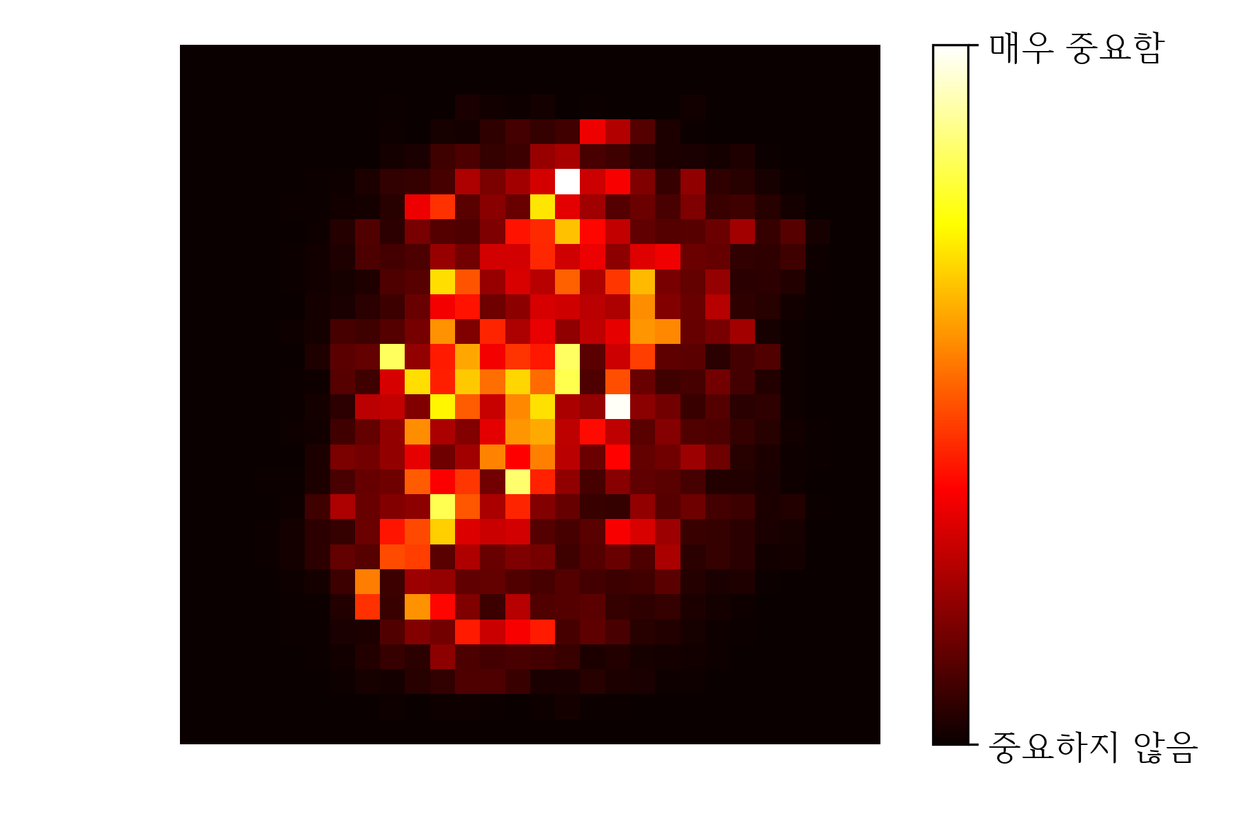
랜덤 포레스트의 장점은 특성(feature)의 상대적인 중요도를 측정하기 쉽다는 것입니다. Scikit-Learn에서는 어떠한 특성을 사용한 노드가 불순도(impurity)를 얼마나 감소시키는지를 계산하여 각 특성마다 상대적 중요도를 측정합니다.
from sklearn.datasets import load_iris

iris = load_iris()
rnd_clf = RandomForestClassifier(n_estimators=500, n_jobs=-1, random_state=42)
rnd_clf.fit(iris["data"], iris["target"])
for name, score in zip(iris["feature_names"], rnd_clf.feature_importances_):
    print(name, score)
sepal length (cm) 0.11249225099876374
sepal width (cm) 0.023119288282510326
petal length (cm) 0.44103046436395765
petal width (cm) 0.4233579963547681
# from sklearn.datasets import fetch_mldata
# mnist = fetch_mldata('MNIST original')
from sklearn.datasets import fetch_openml
mnist = fetch_openml('mnist_784', version=1, return_X_y=True)

rnd_clf = RandomForestClassifier(n_estimators=10, random_state=42)
rnd_clf.fit(mnist[0], mnist[1])

def plot_digit(data):
    image = data.reshape(28, 28)
    plt.imshow(image, cmap = matplotlib.cm.hot,
               interpolation="nearest")
    plt.axis("off")

    plot_digit(rnd_clf.feature_importances_)

    cbar = plt.colorbar(ticks=[rnd_clf.feature_importances_.min(), rnd_clf.feature_importances_.max()])
    cbar.ax.set_yticklabels(['중요하지 않음', '매우 중요함'])

    save_fig("mnist_feature_importance_plot")
    plt.show()
약한 학습기를 여러 개 연결하여 강한 학습기를 만드는 앙상블 방법입니다. 방법의 아이디어는 앞의 모델을 보완해가면서 일련의 예측기를 학습시키는 방법입니다.
과소 적합(underfitted)됐던 학습 데이터 샘플의 가중치는 높이면서 새로 학습된 모델이 학습하기 어려운 데이터에 더 잘 적합되도록 하는 방식입니다.
from sklearn.ensemble import AdaBoostClassifier

# moons 데이터 셋에 AdaBoostClassifier 모델을 학습
X, y = make_moons(n_samples=500, noise=0.30, random_state=42)
X_train, X_test, y_train, y_test = train_test_split(X, y, random_state=42)

ada_clf = AdaBoostClassifier(
    DecisionTreeClassifier(max_depth=1), n_estimators=200,
    algorithm="SAMME.R", learning_rate=0.5, random_state=42)    ## learning_rate를 잘 조절해주는 것도 중요
ada_clf.fit(X_train, y_train)
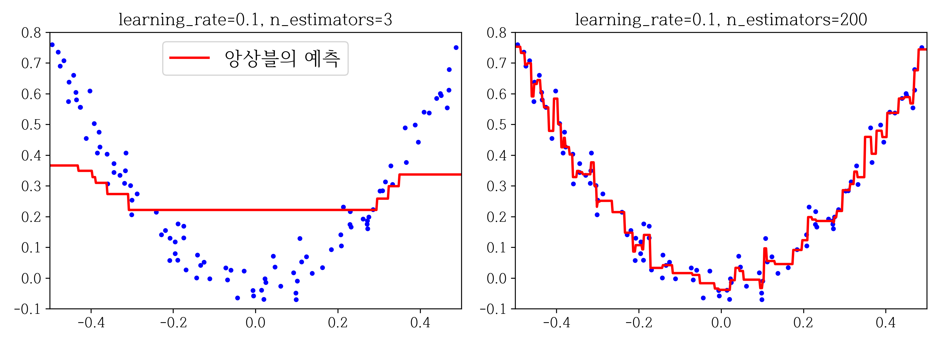
전의 학습된 모델의 오차를 보완하는 방향으로 모델을 추가해주는 방법은 동일합니다. 그래디언트 부스팅은 학습 전 단계 모델에서의 잔여 오차(residual error)에 대해 새로운 모델을 학습시키는 방법입니다.
예제를 통해 알아보겠습니다.
\(y = 3X^2 + 0.05 + noise\)
np.random.seed(42)
X = np.random.rand(100, 1) - 0.5 ## 무작위로 x값 생성
y = 3*X[:, 0]**2 + 0.05 * np.random.randn(100) ## 노이즈가 섞인 값 생성

from sklearn.ensemble import GradientBoostingRegressor

# 낮은 모델 개수
gbrt = GradientBoostingRegressor(max_depth=2, n_estimators=3, learning_rate=0.1, random_state=42)
gbrt.fit(X, y)

# 높은 모델 개수
gbrt_slow = GradientBoostingRegressor(max_depth=2, n_estimators=200, learning_rate=0.1, random_state=42)
gbrt_slow.fit(X, y)
최적의 트리(모델)의 개수를 찾기 위해 조기종료를 사용할 수 있습니다. 간단하게 구현하려면 staged_predict() 메서드를 사용합니다.
stated_predict()를 통해 각 모델의 예측값과 실제값의 MSE를 구한 뒤 error가 가장 낮은 최적의 트리 개수를 찾아 그 개수로 그래디언트 부스팅을 학습시킵니다.
import numpy as np
from sklearn.model_selection import train_test_split
from sklearn.metrics import mean_squared_error

X_train, X_val, y_train, y_val = train_test_split(X, y, random_state=49)

gbrt = GradientBoostingRegressor(max_depth=2, n_estimators=120, random_state=42)
gbrt.fit(X_train, y_train)

## 최적의 트리 개수 찾기
errors = [mean_squared_error(y_val, y_pred)
          for y_pred in gbrt.staged_predict(X_val)]
bst_n_estimators = np.argmin(errors)      ## np.argmin(errors) = 55

## 최적의 트리개수로 다시 학습
gbrt_best = GradientBoostingRegressor(max_depth=2,n_estimators=bst_n_estimators, random_state=42)
gbrt_best.fit(X_train, y_train)
각 모델의 예측값을 가지고 새로운 메타 모델을 학습시켜 최종 예측모델을 만드는 방법입니다.
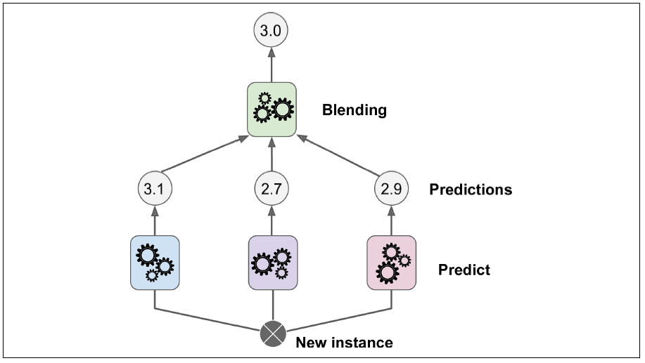
학습 데이터셋에서 샘플링을 통해 서브셋1을 만들고, 이 서브셋을 이용해 각 모델을 학습시킵니다.
서브셋2(나머지 훈련데이터)를 학습시킨 모델에 넣고 각 모델의 예측값을 출력합니다. 그리고 이 예측값들을 input으로 받는 모델을 학습시킵니다. 이 모델을 블렌더(blender) 혹은 메타 학습기(meta learner)라고 부릅니다.
저희는 이번에 앙상블과 랜덤 포레스트를 알아보았습니다. 다음 단원에서는 차원 축소에 대해 살펴보도록 하겠습니다.